Understanding the J Curve: Economic Theory, Applications, and Real World Examples

Exploring the J Curve: Economic principles, real world examples, and implications for businesses & investors.
Introduction to the J Curve
The J Curve is an economic phenomenon that has gained significant attention within various sectors, including trade deficits, private equity, medical conditions, and politics. The term derives its name from the shape of the curve created when representing changes over time. In the context of international economics, a J Curve denotes an initial worsening of a trade deficit following a depreciation, subsequently followed by improvements. This phenomenon can be explained through several economic principles and has significant implications for investors, businesses, and economies.
Under the J Curve Theory
The J Curve theory revolves around the notion that export volumes and import quantities first experience microeconomic changes as prices adjust before substantial shifts occur in trading volumes. In the aftermath of a currency depreciation, the cost of imports for domestic consumers increases, prompting a decrease in the quantity demanded. Meanwhile, foreign buyers find exports from the devalued country more attractive due to their lower prices. These parallel actions ultimately result in an increased trade deficit (or smaller surplus) on the nominal level, forming a J-shaped curve when plotted against time.
The Initial Effects of Devaluation on Trade Balance
When a currency undergoes a depreciation, its total value of imports initially increases due to the higher price levels. However, export volumes remain relatively stagnant during this period because pre-existing trade contracts have yet to be renegotiated or replaced. This results in a worsening nominal trade deficit in the short term.
Long-Term Adjustments
Over time, export quantities begin to grow as foreign buyers find attractive offers from the country with the devalued currency. Conversely, domestic consumers start purchasing fewer imported products due to their increased prices, leading to a narrower trade gap or even a surplus on the nominal level. The lag between the depreciation and the response on the curve is primarily attributed to the adjustment period of existing trade contracts and the time it takes for export quantities to react significantly to price signals.
Significance and Applications Beyond Trade Deficits
The J Curve theory has also found applications in other areas, such as private equity, medical conditions, and politics. For instance, private equity funds historically display a J-shaped pattern when graphed against their performance; they often post early losses but recover with substantial gains over time. Other fields have seen the emergence of similar phenomena, including cholesterol levels and blood pressure in the medical community or engine oil pressure changes in mechanical systems.
Case Study: Japan’s J Curve
The most notable example of a J Curve can be observed in Japan following its sudden currency depreciation in 2013. The country’s trade balance deteriorated due to the increased cost of energy imports and the weaker yen, which led to a record-high nominal trade deficit of 1.3 trillion yen (US$12.7 billion). However, as the yen remained weak and export prices became increasingly competitive, foreign buyers showed growing interest in Japanese goods, ultimately leading to a narrowing trade gap and an eventual surplus.
Implications for Investors and Businesses
The J Curve’s existence has significant implications for investors and businesses. Understanding this economic phenomenon can help them anticipate and adjust strategies accordingly during periods of currency fluctuations and economic instability. Additionally, recognizing the J Curve can provide valuable insights into potential opportunities, risks, and future market trends.
Advantages of a Stronger Currency
The J Curve’s analysis also highlights the importance of having a stronger currency in an international marketplace. A strong currency can help protect businesses from import price increases and boost competitiveness among foreign buyers. However, it is crucial for investors to be aware that the benefits of a stronger currency are not without their challenges, as they might face higher production costs and reduced profitability in export markets.
Managing Risk
Navigating risks associated with currency fluctuations and economic instability can be achieved through various strategies such as diversification, hedging, and maintaining a flexible business model. By understanding the J Curve and its implications for trade balances, investors and businesses can make more informed decisions and mitigate potential risks.
Conclusion:
The J Curve is an essential concept within economics that sheds light on the complex relationship between currency depreciation, international trade, and economic growth. This phenomenon has significant applications in various sectors such as private equity, medical conditions, and politics. By gaining a deeper understanding of the J Curve, investors, businesses, and economists can make informed decisions and anticipate market trends, ultimately driving long-term success and growth.

How the J Curve Operates
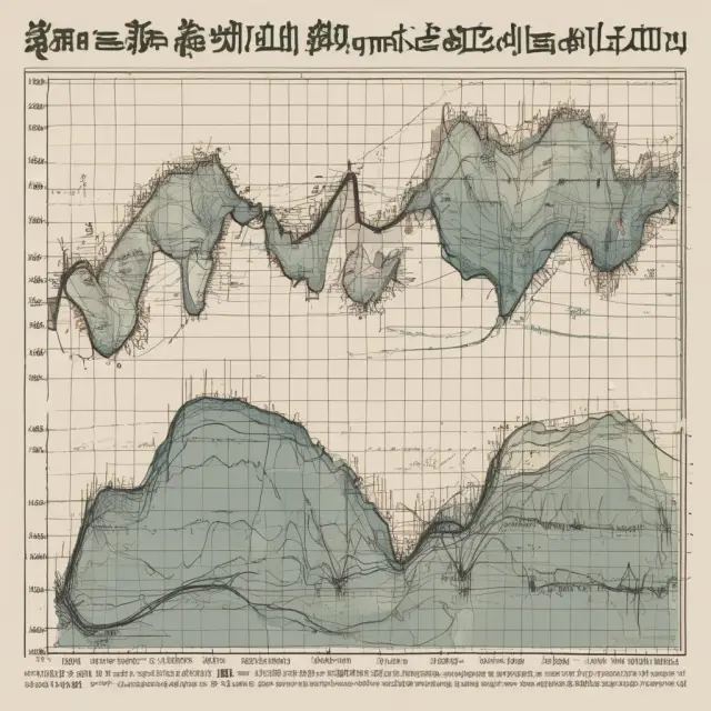
The J Curve economic theory proposes that, following a currency devaluation, the trade deficit of a nation will initially worsen due to higher import prices before eventually shrinking or reversing into a surplus as export quantities adjust. This relationship between currency depreciation and its subsequent impact on trade balances is characterized by a J-shaped curve (Figure 1).
Underlying the J Curve’s dynamics lies the principle that exchange rate shifts initially lead to changes in prices rather than quantities, particularly when it comes to imports and exports. As a result, upon a currency depreciation, import prices will rise substantially for a nation, causing an immediate increase in nominal import volumes (M1). This initial expansion of import purchases is because consumers have not yet shifted their preferences or sourced alternative products domestically. Meanwhile, the quantity of exports remains largely unchanged initially, as existing contracts are honored and export partners adjust to the new price conditions. Consequently, a larger nominal trade deficit emerges due to these factors.
Figure 1: The J Curve illustrates the initial worsening of a nation’s trade balance following a currency depreciation (devaluation), eventually resulting in a shrinking deficit or even surplus as export quantities increase and import volumes decrease.
However, over time, as quantities begin to adjust, exports experience growth due to their more competitive pricing for foreign buyers. This shift leads to an increase in total nominal export volumes (M2). On the other hand, domestic consumers start reducing their demand for imports due to their higher prices. As a result, import purchases decrease, and the nation’s trade balance improves, eventually shrinking or reversing into a surplus.
The time lag between the currency devaluation and the response on the J Curve can be attributed to various factors such as the impact of exchange rate fluctuations on the total value of imports (M1). Even after a currency experiences a depreciation, import prices will likely increase significantly before export volumes adjust. However, over the long-term, large numbers of foreign consumers may boost their purchases of products from the country experiencing a currency devaluation as these goods now become cheaper relative to domestically-produced items.
It’s essential to note that the J Curve applies not only to trade balances but also to various aspects of economics and business. For instance, private equity funds often exhibit characteristics of a J Curve, with poor initial returns followed by significant gains due to events like mergers and acquisitions (M&A), initial public offerings (IPOs), and leveraged recapitalization. Other areas where the J Curve concept can be applied include medicine, engineering, and politics.
In summary, the J Curve theory highlights the importance of understanding the relationship between currency depreciation and its impact on trade balances. By recognizing how prices and quantities adjust over time, investors and economists alike can better anticipate market behavior and make informed decisions in the face of exchange rate changes.

Initial Effects of a Devaluation on Trade Balance
The J Curve theory, named for its distinctive shape when plotted as a line graph, is an essential economic concept that describes the reaction of a country’s trade deficit to currency depreciation. According to this theory, after the initial devaluation, the nominal trade balance will worsen due to increased import volumes and static export quantities.
When a nation experiences a currency depreciation, prices on imports become more expensive for domestic consumers. This cost increase causes an uptick in import purchases before the quantity of these imports begins to decrease over time. The higher import volume, combined with unchanged export quantities, leads to a worsening nominal trade deficit—the characteristic initial dip at the base of the ‘J.’
The J Curve theory assumes that prices adjust more quickly than quantities, resulting in a short-term increase in imports due to their temporarily lower relative cost. After this phase, the quantity of exports begins to grow as foreign buyers are drawn by the competitiveness of the depreciated currency. This eventually leads to a reduced trade deficit or even a surplus as export volume expands and import quantities contract.
In essence, the J Curve demonstrates how initial economic reactions may mask underlying forces that eventually lead to long-term adjustments with profound implications for both traders and investors. The theory’s insights can be applied beyond currency devaluations, providing valuable context for understanding various aspects of economics and finance, including private equity investments, medical conditions, and political unrest.
In summary, the J Curve is an invaluable economic concept that describes the short-term worsening trade deficit following a currency depreciation and its eventual reversal as prices and quantities adjust. The theory’s insights extend far beyond currency markets, illuminating the complex dynamics of various aspects of economics and finance.
As we delve deeper into the J Curve in subsequent sections, we will explore real-world examples and discuss strategies for managing risk during periods of economic instability and currency fluctuations.
Long-Term Adjustments to a J Curve
The long-term adjustments to the J Curve refer to the shifts in export volumes, import purchases, and overall trade balance that occur after an initial devaluation of a currency. The J Curve is rooted in the notion that trading volumes of imports and exports first experience microeconomic changes as prices adjust before quantities do. As time passes, there are significant modifications in both import volumes and export quantities.
The J Curve’s long-term impact on a country’s trade balance primarily stems from the fact that as exported goods become more competitively priced due to their currency depreciation, foreign buyers increasingly seek these products. Conversely, domestic consumers gradually reduce their purchases of imported goods because they are now relatively more expensive compared to domestically produced alternatives. These parallel shifts in demand result in a more favorable trade balance over time.
However, it is important to note that the J Curve does not imply immediate changes following devaluation. The impact on the economy can be slow to manifest as previously established trade contracts and agreements play out, leading to a lag between the currency adjustment and the response on the curve. The length of this adjustment period depends on factors like market dynamics, economic structures, and the magnitude of the exchange rate change.
When a country experiences an appreciation in its currency, the J Curve takes on an inverted shape as imports become less attractive to domestic consumers, while exports become more expensive for foreign buyers, leading to decreased import volumes and increased export volumes. These adjustments eventually lead to a more favorable trade balance or surplus.
In conclusion, the J Curve’s long-term adjustments play a crucial role in understanding how changes in exchange rates ultimately shape a country’s trade dynamics. This economic theory provides valuable insight into the impact of currency depreciation and appreciation on import volumes, export quantities, and overall trade balances. It is essential for investors, policymakers, and businesses to comprehend these long-term shifts to make informed decisions in an increasingly globalized economy.

Applications of the J Curve Beyond Trade Deficits
The J Curve theory, initially introduced as a framework for explaining the relationship between trade deficits and currency depreciation, has proven to be an influential concept in various fields beyond economics. This section will illustrate three non-traditional applications: private equity, medical conditions, and politics.
1. Private Equity:
The J Curve theory is often used in the context of private equity investment funds to describe the performance trend over time. In their early years, these funds may suffer negative returns due to high management fees and other costs. However, they eventually begin to yield significant gains from successful investments such as mergers and acquisitions (M&A), initial public offerings (IPOs), and leveraged recapitalizations. The J Curve in private equity represents the concept of an initial paradoxical response followed by a strong positive outcome, which can be seen when graphing returns against time.
2. Medical Conditions:
J Curves are also prevalent in medical research, especially when it comes to studying the relationship between certain health conditions and their associated risks. For instance, consider cholesterol levels and the likelihood of cardiovascular disease. The X-axis can represent cholesterol levels, while the Y-axis indicates the risk of developing heart disease. Initially, an increase in cholesterol may seem to correspond with a higher risk for cardiovascular disease due to its association with plaque buildup in arteries. However, after reaching a certain threshold, the risk then significantly decreases due to the body’s ability to adapt and compensate. This nonlinear relationship is often described as a J Curve.
3. Politics:
Political scientists have employed the J Curve theory to analyze the phenomenon of political revolutions. James Chowning Davies, an American sociologist, argued that riots are a reaction to a sudden reversal in fortunes after a long period of economic growth—a concept known as relative deprivation. A J-shaped relationship can be observed when graphing social unrest against the level of economic development, with instability peaking at a certain stage before eventually subsiding. The theory suggests that as societies reach an inflection point in their economic trajectory, they may experience significant upheaval until the situation stabilizes once more.
Understanding the J Curve’s versatility showcases its importance not only to economists but also to researchers in various fields. Whether examining financial investments, medical conditions, or political instability, this nonlinear pattern continues to reveal valuable insights into complex systems and relationships.

Real World Example: Japan’s J Curve
The J Curve, an economic theory that describes the worsening of a country’s trade deficit following currency depreciation, was put to the test in Japan after its currency took a significant hit in 2013. The yen experienced a dramatic drop against the US dollar, with the exchange rate reaching a six-year low of 100 USD per JPY. This devaluation led to a surge in imports and an initial worsening of Japan’s trade deficit, illustrating the J Curve effect in real life.
Following the yen’s sharp decline, imported goods became cheaper for Japanese consumers, causing a rise in demand for foreign products. In contrast, export prices remained stable until existing trade contracts were fulfilled. This price disparity created an imbalance that saw Japan’s nominal trade deficit swell to a record-breaking 1.3 trillion yen (approximately US$12.7 billion).
However, the story doesn’t end there. As quantities began to adjust with time, exports gained attractiveness for foreign buyers due to their relatively lower prices compared to domestically produced goods. Simultaneously, Japanese consumers shifted towards domestic products as imported items grew more expensive, causing import volumes to decrease. This dynamic led to a reduction in the trade deficit and eventually a reversal into a surplus.
The J Curve’s implications extend beyond trade deficits. It can be observed in various fields such as private equity, medical conditions, and politics. The theory can illustrate how private equity funds initially suffer losses due to investment costs and management fees but eventually yield returns through strategic investments like mergers and acquisitions (M&A), initial public offerings (IPOs), or leveraged buyouts. In medicine, J Curves represent the likelihood of cardiovascular diseases in patients with specific conditions, such as cholesterol levels or blood pressure, when plotted against time.
In summary, Japan’s experience in 2013 provides a real-world example of how the J Curve operates and its eventual impact on trade balances after currency depreciation. Though it may take some time for quantities to adjust, the theory holds that the worsening trade deficit will eventually reverse as exports grow more competitive and imports decrease in response to price changes.

Economic Implications for Investors and Businesses
Understanding the J Curve has far-reaching implications for both investors and businesses, particularly in the context of currency depreciation or appreciation. The J Curve explains how trade balances evolve when a country’s currency undergoes a significant change, be it through devaluation or revaluation. This knowledge is crucial for making sound investment decisions, assessing trade strategies, and forecasting economic trends.
When a nation experiences currency depreciation, the J Curve demonstrates that initial trade deficits may worsen as prices of imports surge. However, as quantities eventually adjust over time, export volumes increase, and domestic demand for imports decreases, the country’s trade balance shifts towards a surplus or smaller deficit.
This theory is not only applicable to trade balances; it can also be observed in various sectors, including private equity, medical conditions, and politics. For instance, private equity funds may initially show negative returns post-launch but eventually yield positive results through strategic acquisitions and IPOs. In the medical field, J Curves have been used to model how cardiovascular diseases develop with varying degrees of risk for different conditions.
For investors, understanding the J Curve can help in anticipating changes in trade balances during currency fluctuations. As prices of exports become more attractive to foreign buyers and imports become relatively more expensive, adjustments to investment portfolios and trading strategies may be necessary.
Businesses, too, benefit from this knowledge as they prepare for shifts in the demand for their products and services, both domestically and internationally. By understanding the J Curve’s impact on trade balances, businesses can adapt to changes in currency values and remain competitive during periods of economic instability.
One real-world example of the J Curve is Japan’s experience following its 2013 depreciation of the yen. Initially, the country’s trade deficit worsened due to increased energy imports and higher prices for imported goods. However, as time passed, export volumes began to expand, and import demand decreased. This shift led to a significant improvement in Japan’s trade balance, with a reduction in its record-breaking 1.3 trillion yen deficit.
The J Curve offers valuable insights into the dynamics of economic change and how they can affect various sectors and industries. By staying informed about this economic phenomenon, investors and businesses alike can make more informed decisions during periods of currency fluctuations and geopolitical uncertainty.

Advantages of a Stronger Currency in a Global Economy
The J Curve theory is most famously known for its impact on trade balances, but it can also offer significant advantages when it comes to having a stronger currency in the global economy. A stronger currency can positively influence businesses and investors alike by increasing their purchasing power, competitiveness, and overall financial stability.
First and foremost, a stronger domestic currency leads to increased purchasing power for both individuals and corporations. With more value from each unit of their currency, they can buy goods and services at lower prices or expand their reach into international markets where the cost of production might be cheaper. This can lead to improved profit margins and increased competitiveness in the global marketplace.
A strong currency also translates to a stronger balance sheet for a country. When a country’s currency strengthens, it results in reduced debt costs because foreign investors must pay more to purchase that country’s securities or bonds. This means that interest payments made in a stronger currency cost less in domestic currency terms. Furthermore, having a strong currency makes a country an attractive destination for foreign direct investment (FDI) and portfolio investments as well. This inflow of capital can contribute to economic growth by generating jobs, increasing exports, and fostering technological innovation.
In the context of international trade, a stronger currency provides competitive advantages in industries where a country has a comparative advantage or is a significant global player. For instance, countries that are rich in natural resources may benefit from having a strong currency as it allows them to sell their raw materials at higher prices without facing substantial competition due to lower production costs. Similarly, companies in sectors with high value-added products can also prosper with a stronger domestic currency since their products become more attractive to foreign buyers.
However, there are risks associated with having a strong currency. A currency that is too strong could potentially lead to a loss of competitiveness for industries that rely heavily on exports or face strong competition from foreign producers. In such cases, companies may consider offshoring production to countries where labor costs are lower or implementing productivity improvements to maintain their edge in the global marketplace.
Despite these potential challenges, the overall benefits of a stronger domestic currency can far outweigh the disadvantages for many businesses and investors. By understanding the J Curve’s implications for trade balances as well as its advantages for having a stronger currency, we gain valuable insights into how economies and currencies interact in today’s interconnected world.
FAQs About the Advantages of a Stronger Currency
Question: How does a stronger domestic currency impact imports and exports?
Answer: A stronger domestic currency increases the price of imports for buyers in that country, making them less attractive while exports become more competitive as they become cheaper for foreign buyers. This can lead to a shift in the trade balance towards a surplus or smaller deficit.
Question: What are some industries that benefit from having a strong currency?
Answer: Industries with high value-added products, natural resources, and significant global presence can all benefit from having a stronger domestic currency due to increased competitiveness and purchasing power.
Question: What risks come with having a strong currency?
Answer: A currency that is too strong could lead to decreased competitiveness for industries that rely heavily on exports or face strong competition from foreign producers. In such cases, companies may consider offshoring production or implementing productivity improvements to maintain their edge in the global marketplace.

Managing Risk in the Context of a J Curve
Understanding and managing risk in the context of the J Curve requires a nuanced approach given its inherent complexities and potential impact on economic stability. The J Curve, a theory that describes how a country’s trade balance responds to currency fluctuations, is an essential concept for investors, businesses, and policymakers alike. While the J Curve offers valuable insights into market dynamics, it can also introduce new challenges when managing risk during periods of currency instability.
The J Curve demonstrates that following a devaluation or appreciation of a currency, there will be an initial adjustment phase characterized by increased uncertainty and heightened risk. During this period, trade balances may deteriorate as the market adapts to new price signals and quantities gradually shift. This instability can present challenges for businesses and investors, particularly those with significant exposure to international markets.
One potential strategy for managing risk during a J Curve event is hedging. By employing financial derivatives such as currency options or futures contracts, market participants can protect themselves against adverse price movements in the foreign exchange market. Hedging strategies enable organizations and individuals to lock in favorable exchange rates while mitigating the risks associated with currency volatility.
Another strategy involves diversifying risk across multiple markets, geographies, or industries. Diversification helps to minimize exposure to a single market that could be subject to significant currency fluctuations or economic instability. By spreading investments and business operations across various markets, companies can reduce their overall sensitivity to currency movements and thereby insulate themselves from potential J Curve effects.
Monitoring global economic indicators and market trends is also crucial for managing risk in a J Curve context. By staying informed about key data releases, political developments, and other factors that may impact exchange rates and trade balances, investors and businesses can make more informed decisions regarding their investment strategies and risk management tactics.
Furthermore, building strong relationships with suppliers and customers located in markets subject to J Curve dynamics can be essential for managing risk. By fostering robust business partnerships, organizations can improve communication channels and enhance their ability to adapt quickly to changing market conditions. In the context of a J Curve event, having reliable and flexible suppliers or customers can help mitigate the risks associated with currency fluctuations and other economic uncertainties.
Finally, understanding the long-term implications of the J Curve is key for managing risk effectively. By recognizing that initial deterioration in trade balances may be temporary as markets adjust to new price signals and quantities shift, investors and businesses can maintain a longer-term perspective and avoid panic selling or unnecessary risk aversion.
In conclusion, the J Curve presents unique challenges for managing risk during periods of currency instability. Strategies such as hedging, diversification, monitoring economic indicators, and building strong business relationships can help organizations effectively navigate the complexities of this economic theory. By staying informed and adaptive, investors and businesses can minimize risks associated with J Curve dynamics and capitalize on the opportunities that may arise in the global marketplace.

Conclusion: The Role of the J Curve in Modern Economics
The J Curve is an intriguing economic theory that sheds light on how currency depreciation or appreciation can significantly impact trade balances, both in the short term and long term. Understanding this phenomenon not only offers valuable insights into macroeconomic principles but also provides crucial knowledge for investors, businesses, and policymakers operating in an increasingly interconnected global economy.
In essence, a J Curve refers to the characteristic letter “J” shape that appears when the nominal trade balance is plotted on a graph after currency devaluation or revaluation. The initial response of a depreciated currency is the worsening of a country’s trade deficit, as import prices increase and export quantities remain relatively stable due to existing contracts. However, over time, exports eventually gain momentum from their more attractive pricing and increased demand from foreign buyers. Simultaneously, domestic consumers curb their imports, resulting in an improvement or reversal of the trade deficit into a surplus.
The J Curve theory extends beyond the realm of trade balances; it is also relevant to various sectors such as private equity, medicine, and politics. For instance, private equity funds often follow a J Curve pattern, with initial losses due to costs and management fees but eventually producing significant returns through M&A, IPOs, and other strategic moves. Medical conditions like cholesterol levels or blood pressure demonstrate the J Curve in their relationship with the likelihood of cardiovascular disease. Additionally, the J Curve has been used to explain political revolutions as a response to sudden reversals in economic fortunes after extended periods of growth.
A practical example of the J Curve is seen in Japan’s trade balance following the depreciation of its currency in 2013. The yen’s decline led to an initial worsening of the country’s trade deficit due to higher import costs and unchanged export levels. However, over time, Japanese exports gained traction from their more competitive pricing, while imports decreased as domestic consumers adjusted to the increased prices.
The J Curve is a powerful concept that plays an essential role in shaping economic strategies and forecasts for investors and businesses operating in international markets. In times of currency volatility or uncertainty, understanding the principles behind the J Curve can provide valuable insights into the potential impact on trade balances and the economy as a whole. Moreover, being aware of this phenomenon allows for the implementation of effective risk management strategies to navigate through these periods of economic change.
The J Curve’s significance goes beyond just understanding its effects on trade balances; it also illustrates the complex interplay between prices and quantities in the global economy, and highlights the importance of patience and long-term perspective for investors and businesses alike.
FAQs About the J Curve
What exactly is a J Curve in economics?
A J Curve is an economic theory that indicates how a country’s trade deficit or surplus evolves following currency depreciation or appreciation, respectively. When plotted as a line graph, the resulting shape resembles the letter ‘J,’ with initial worsening and subsequent improvement in the trade balance.
Why does the J Curve occur?
The J Curve arises due to the time lag between currency depreciation (or appreciation) and the adjustment of import and export volumes in response to price changes. Initially, imports increase in value but not quantity, causing a deterioration in the trade balance before quantities eventually respond and the balance improves.
What conditions must be met for a J Curve to form?
The theory assumes that prices change immediately upon currency depreciation or appreciation, while import and export volumes adjust gradually. Additionally, the theory requires that the impact of price changes on imports and exports is felt differently, with imports being more sensitive to price fluctuations in the short term.
Can the J Curve be observed outside of trade balances?
Yes! The concept of a J Curve can be applied to private equity funds, medical conditions, and political revolutions, where an initial paradoxical response is followed by a strong response in the expected direction. These applications share the common thread of a time lag between an event and its ultimate effect on outcomes.
What is the significance of the J Curve for investors?
The J Curve provides valuable insights into how currency depreciation (or appreciation) can influence trade balances and impact the performance of foreign investments. Understanding this theory can help investors make more informed decisions regarding their portfolios, particularly when investing in markets undergoing currency changes.
What real-world examples demonstrate the J Curve at work?
A prominent example of a J Curve occurred in Japan following its sudden yen depreciation in 2013. Despite initial worsening of the trade balance due to increased import and decreased export volumes, the country eventually saw an improvement in its trade position over time as quantities adjusted to price changes.
How long does it take for a J Curve to manifest?
The length of time required for a J Curve to appear depends on various factors such as market conditions, the responsiveness of import and export volumes to price changes, and government policies aimed at managing currency fluctuations. In general, longer-term trends are more likely to exhibit a J Curve shape than short-term price movements.
 Next entry · No. 2,586Jean-Baptiste Say: The Influential French Economist Behind Say’s Law
See also
-
 No. 4,287
06 Jun 2025
19 min
Understanding Rational Expectations Theory: Predicting Future Economic Outcomes
Economics
No. 4,287
06 Jun 2025
19 min
Understanding Rational Expectations Theory: Predicting Future Economic Outcomes
Economics -
 No. 2,578
18 Jan 2025
22 min
The January Barometer: An In-Depth Look at this Market Indicator and its Implications for Institutional Investors
Finance Policy
No. 2,578
18 Jan 2025
22 min
The January Barometer: An In-Depth Look at this Market Indicator and its Implications for Institutional Investors
Finance Policy -
 No. 2,372
31 Dec 2024
20 min
Mastering Indifference Curve Analysis: A Comprehensive Guide for Institutional Investors
Business Finance
No. 2,372
31 Dec 2024
20 min
Mastering Indifference Curve Analysis: A Comprehensive Guide for Institutional Investors
Business Finance -
 No. 1,646
17 Oct 2024
27 min
Understanding Forward Exchange Contracts: A Comprehensive Guide for Institutional Investors
Finance Policy
No. 1,646
17 Oct 2024
27 min
Understanding Forward Exchange Contracts: A Comprehensive Guide for Institutional Investors
Finance Policy -
 No. 5,783
07 Oct 2025
19 min
Understanding the Concept and Impact of Working-Age Population
Economics
No. 5,783
07 Oct 2025
19 min
Understanding the Concept and Impact of Working-Age Population
Economics -
 No. 5,572
20 Sep 2025
18 min
Understanding the Wage-Price Spiral and Its Impact on Inflation
Finance Policy
No. 5,572
20 Sep 2025
18 min
Understanding the Wage-Price Spiral and Its Impact on Inflation
Finance Policy