Three-Sigma Limits: Setting Control Limits for Financial Processes and Investments
Learn about Three-Sigma Limits - a statistical approach for setting control limits in financial processes, investments and quality assurance.
Understanding Three-Sigma Limits: The Basics
Three-sigma limits, also known as 3-sigma limits, is a statistical concept that signifies data within three standard deviations from the mean. In business contexts, this term refers to processes functioning optimally and producing high-quality items. Three-sigma limits are instrumental in establishing upper and lower control limits for statistical quality control charts. Control charts, first introduced by Walter A. Shewhart, a renowned American physicist, engineer, and statistician, determine the presence of controlled or uncontrolled process variation.
Control charts, also called Shewhart charts, operate based on the idea that variability exists even in perfectly designed processes. These charts serve to distinguish between random causes of variations (in-control) and special causes (out-of-control). Statisticians and analysts employ a vital statistical measurement known as standard deviation, or sigma, to evaluate these variations.
Sigma is the measure of variability that quantifies how far a data point diverges from the mean. In finance, investors often apply standard deviation to assess risk and volatility in investments, referred to as historical volatility.
The normal bell curve illustrates the significance of three-sigma limits. A data point’s position on this graph indicates its proximity to the average or mean. Data points close to the mean have low values; high values represent widespread data that deviate significantly from the mean.
Consider a manufacturing firm that runs ten tests to evaluate its product quality. The obtained data points are 8.4, 8.5, 9.1, 9.3, 9.4, 9.5, 9.7, 9.7, 9.9, and 9.9. To calculate the mean, sum up all data points (8.4 + 8.5 + 9.1 + 9.3 + 9.4 + 9.5 + 9.7 + 9.7 + 9.9 + 9.9) and divide by the total number of observations (10), resulting in a mean of 9.34.
To determine variance, sum up the squared difference between each data point and the mean: 0.8836, 0.7056, 0.0576, etc. Divide this sum by the total number of observations to find the variance (2.564 / 10 = 0.2564).
Calculate standard deviation by finding the square root of the variance (√0.2564 = 0.5064). Three-sigma limits are determined by adding three standard deviations to the mean: (3 x 0.5064) + 9.34 = 10.9. Since no data point exceeds this value, the manufacturing testing process has not attained three-sigma quality levels yet.
Three-sigma limits signify a controlled process where approximately 99.73% of all data points fall within the predefined range of three standard deviations from the mean.
The Bell Curve and Normal Distribution
Three-sigma limits are based on the concept of normal distribution or Gaussian distribution, commonly known as a bell curve. A normal distribution is a continuous probability distribution describing a large collection of independent random variables, each having the same probability density function. This distribution is defined by its mean (average) and standard deviation. In statistics, 68% of data falls within one standard deviation of the average; 95% falls within two standard deviations; and an impressive 99.73% falls within three standard deviations.
The significance of a normal distribution lies in its symmetry around the mean, where the mean is also the mode (the most frequently occurring value). The curve is bell-shaped, with values decreasing gradually as we move away from the mean towards the tails. Data points at the far ends of the tail are less common than those closer to the average.
The importance of a normal distribution in three-sigma limits arises from understanding how far data can deviate from the mean before being considered an outlier or uncontrolled point, which might indicate a special cause requiring corrective action. When we calculate three standard deviations above and below the mean, we obtain a range where over 99.73% of observations fall. In other words, the process is expected to remain within these limits most of the time, ensuring operational efficiency and consistent product quality.
Calculating the mean and variance are fundamental steps in determining three-sigma limits. In our previous example, we calculated the mean and variance from a series of 10 tests in a manufacturing company. We established that the mean was 9.34 and the standard deviation was 0.5064. Three standard deviations above the mean would be (3 x 0.5064) + 9.34 = 10.9, while three standard deviations below the mean is -(3 x 0.5064) + 9.34 = 7.8. By calculating these limits, we can monitor and evaluate the performance of our manufacturing process or investment portfolio against the established norms.

Calculating the Mean and Variance
Three-sigma limits is a critical statistical concept used to determine control limits for processes in various industries, including manufacturing and finance. It’s based on understanding the normal distribution and bell curve. Let us delve deeper into calculating the mean and variance—two essential components of three-sigma limits—using a step-by-step process.
Mean (Average) Calculation
To calculate the mean, or average, we need to follow these steps:
- Add up all the data points in the dataset.
- Divide the sum by the total number of observations.
For instance, consider a set of 10 test results from a manufacturing process: {8.4, 8.5, 9.1, 9.3, 9.4, 9.5, 9.7, 9.7, 9.9, 9.9}.
To find the mean, perform these calculations:
Step 1: Add up all data points: 8.4 + 8.5 + 9.1 + 9.3 + 9.4 + 9.5 + 9.7 + 9.7 + 9.9 + 9.9 = 93.4
Step 2: Divide the sum by the total number of observations (n): Mean = 93.4 / 10 = 9.34
Variance Calculation
The variance is a measure of spread or dispersion in the data set around the mean. To calculate the variance, follow these steps:
- Subtract each data point from the mean (finding the difference).
- Square each difference.
- Find the sum of all squared differences.
- Divide the sum by the total number of observations (n).
Let’s calculate the variance for our manufacturing process example:
Step 1: Subtract each data point from the mean, finding the differences: {-0.9, -0.8, -0.2, -0.1, -0.1, 0, 0.3, 0.3, 0.6, 0.6}
Step 2: Square each difference: {0.81, 0.64, 0.04, 0.01, 0.01, 0, 0.9, 0.9, 3.61, 3.61}
Step 3: Find the sum of all squared differences: 0.81 + 0.64 + 0.04 + 0.01 + 0.01 + 0 + 0.9 + 0.9 + 3.61 + 3.61 = 7.1
Step 4: Divide the sum by the total number of observations (n): Variance = 7.1 / 10 = 0.7056 or approximately 0.71
Now, to find the standard deviation, take the square root of the variance: Standard Deviation = √(Variance) = √(0.7056) ≈ 0.8426
The mean is 9.34, and the standard deviation is approximately 0.8426. With these values, we can now calculate three-sigma limits for our manufacturing process or any other industry application.
Determining Standard Deviation
Three-sigma limits rely on statistical calculations to identify if a process is under control or not. One crucial metric in this calculation is standard deviation, which measures the spread between a given data set and its mean value. In this section, we’ll discuss how to calculate standard deviation, its significance in three-sigma limit calculation, and an example to better understand the concept.
Understanding Standard Deviation
Standard deviation (σ) is a measure of dispersion or variability within a data set. It determines the spread between each data point and the mean value by calculating the square root of variance (average of squared differences from the mean). For investors, standard deviation represents historical volatility, providing insight into the expected range of possible outcomes for an investment’s returns.
The Bell Curve Connection
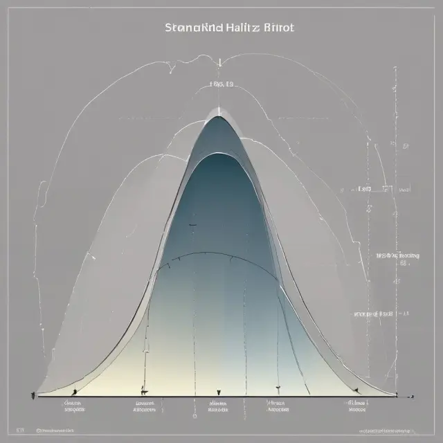
To appreciate three-sigma limits better, we must first understand the normal distribution and its accompanying bell curve. This graphical representation shows how a data set is distributed around the mean with most values clustered near the center and fewer occurrences further away from it. Three-sigma limits come into play by setting control limits at three standard deviations above and below the mean, representing approximately 99.73% of all data points.
Calculating Standard Deviation
To calculate the standard deviation for a given dataset, follow these steps:
- Find the dataset’s mean value by summing up all values and dividing by the total number of observations (sample size).
- Subtract the mean from each observation to find the difference between the mean and each observation.
- Square each difference obtained in step 2 and sum up these squared differences.
- Divide the sum of squared differences by the sample size minus one (n-1) to find the variance.
- Finally, take the square root of the variance to get the standard deviation.
Example:
Let’s take a look at a simple example involving a dataset containing ten measurements for a manufacturing process: 8.4, 8.5, 9.1, 9.3, 9.4, 9.5, 9.7, 9.7, 9.9, and 9.9.
Step 1 – Calculate the mean value:
Mean = (Sum of observations) / Number of observations = (8.4 + 8.5 + 9.1 + 9.3 + 9.4 + 9.5 + 9.7 + 9.7 + 9.9 + 9.9) / 10
Mean = 93.4 / 10
Mean = 9.34
Step 2 – Subtract the mean from each observation:
8.4 – 9.34 = -0.9, 8.5 – 9.34 = -0.84, 9.1 – 9.34 = -0.24, …
Step 3 – Square each difference:
(-0.9)² = 0.81, (-0.84)² = 0.7056, (-0.24)² = 0.0576, …
Step 4 – Sum up these squared differences:
Σ(xi-x̄)² = 0.81 + 0.7056 + 0.0576 + …
Σ(xi-x̄)² = 2.564
Step 5 – Divide the sum by the sample size minus one:
Variance (σ²) = Σ(xi-x̄)² / (n-1)
Variance (σ²) = 2.564 / 9
Variance (σ²) = 0.285
Step 6 – Calculate standard deviation:
Standard deviation (σ) = √(Σ(xi-x̄)² / (n-1))
Standard deviation (σ) = √0.285
Standard deviation (σ) = 0.534
Three-sigma limits calculation requires three standard deviations above and below the mean, which is calculated as follows: 3 x Standard Deviation (Σ) + Mean. In our example, three sigma above the mean results in a value of 12.814, while three sigmas below the mean equals 5.876. The manufacturing firm can use this information to check if its process falls within these three-sigma control limits, ensuring an acceptable level of quality and efficiency.
Three-Sigma Control Limits: Setting Up the Process
The concept of three-sigma control limits refers to the process where data falls within three standard deviations from a mean, forming a fundamental part of statistical quality control. The term ‘three-sigma’ is derived from Shewhart’s work and signifies a rational and economic guide for achieving minimal economic loss. These limits help in monitoring a manufacturing or business process to determine the presence of special causes, ensuring efficiency and high-quality production.
To calculate three-sigma limits, first, we determine the mean (average) and variance of a given set of data points. After obtaining these values, we can then calculate the standard deviation as the square root of the variance. Three-sigma is obtained by adding or subtracting three times the standard deviation to the mean, defining the upper and lower control limits for the process.
For instance, let us consider a manufacturing firm that runs 10 tests on its products to assess product quality. The data points collected from these tests are: 8.4, 8.5, 9.1, 9.3, 9.4, 9.5, 9.7, 9.7, 9.9, and 9.9. First, we calculate the mean:
(8.4 + 8.5 + 9.1 + 9.3 + 9.4 + 9.5 + 9.7 + 9.7 + 9.9 + 9.9) / 10 = 9.34
Next, we determine the variance:
Variance = Sum of the squared differences between each data point and the mean divided by the total number of observations
(8.4 – 9.34)² + (8.5 – 9.34)² + … + (9.9 – 9.34)² / 10 = 2.564
Now, we calculate the standard deviation as the square root of the variance:
Standard Deviation = √Variance = √2.564 = 0.5064
The three-sigma limit is obtained by adding or subtracting three standard deviations to the mean:
Three-Sigma Upper Control Limit (UCL) = Mean + Three Standard Deviations = 9.34 + (3 x 0.5064) = 10.9
Three-Sigma Lower Control Limit (LCL) = Mean – Three Standard Deviations = 9.34 – (3 x 0.5064) = 7.8
In the example above, none of the data points exceeded the three-sigma upper control limit of 10.9 or fell below the lower control limit of 7.8, indicating that the manufacturing process is under statistical control and producing items within acceptable quality levels.
It’s important to note that processes operating at the three-sigma level are considered highly efficient and in a state of statistical control, with less than 1% of data points falling outside the upper or lower control limits. In summary, understanding three-sigma control limits is crucial for monitoring process efficiency, quality control, and risk assessment.
Applications in Manufacturing and Quality Assurance
Three-Sigma Limits play an essential role in manufacturing industries by ensuring efficient processes and high product quality. In quality assurance, statistical process control (SPC) relies heavily on the application of three-sigma limits to establish control limits for production processes. The use of three-sigma limits enables manufacturers to identify any potential out-of-control conditions that could impact the consistency and reliability of their products.
The concept behind three-sigma limits originates from the normal distribution, also known as the bell curve. The normal distribution is a continuous probability distribution that represents various naturally occurring random variables, including product measurements in manufacturing environments. By understanding this distribution, manufacturers can identify the likelihood of data points falling within certain ranges and set appropriate control limits.
To determine three-sigma limits for a process, the first step involves calculating the mean (average) and variance. The mean represents the central point around which the majority of the data is distributed, while the variance measures the spread between individual data points and the mean. Calculating the standard deviation from the mean is crucial, as it helps establish the three-sigma limits for a process.
Calculating the Mean and Variance
To illustrate how three-sigma limits are calculated in a manufacturing context, consider a hypothetical manufacturing operation producing ball bearings with a target diameter of 25mm. The following steps outline the process:
- Measure the diameter of each ball bearing from ten randomly selected samples.
- Calculate the mean (average) by summing all measurements and dividing by ten (10).
- Calculate the variance by finding the differences between each measurement and the mean, squaring those differences, summing them up, and then dividing the result by nine.
- Determine the standard deviation by taking the square root of the calculated variance.
- Multiply the standard deviation by three to get the three-sigma limits (upper and lower).
Once these limits are established, manufacturers can use control charts to monitor their processes continually and identify any data points that fall outside the defined range. By setting up a control chart with the upper and lower control limits, manufacturing personnel can quickly assess whether the process is in a state of statistical control or if special causes of variation require further investigation.
Case Studies
One well-known example of the application of three-sigma limits is the production process of ball bearings at the Ford Rouge plant during the 1920s. Walter A. Shewhart, a statistician working for the company, implemented SPC in their manufacturing processes. Using three-sigma control limits, Ford was able to reduce the number of defective ball bearings significantly, saving millions of dollars and improving overall product quality.
Another notable example is from the automobile industry, where General Motors (GM) used statistical process control to monitor its assembly line operations during the 1930s. The application of three-sigma limits helped reduce assembly time and increase production efficiency by minimizing the occurrence of defects and downtime caused by out-of-control conditions.
In conclusion, understanding and applying three-sigma limits is essential for manufacturing industries to maintain quality control in their processes and produce high-performing products. By monitoring data points within their control chart, manufacturers can quickly identify any potential issues and take corrective actions before they escalate into more significant problems. The implementation of three-sigma limits has been proven successful through various case studies, such as those from Ford and General Motors, making it a cornerstone in the world of continuous improvement and quality assurance.
Next: Understanding Three-Sigma Limits: The Basics (Part I) >
It focuses on the concept of three-sigma limits in manufacturing and quality assurance, providing real-life case studies and an explanation of how to calculate these limits in a manufacturing context.

Investment Analysis: Using Three-Sigma Limits
Three-sigma limits are not only useful in manufacturing processes but also in investment portfolio management and risk assessment. By applying statistical analysis and the concept of three-sigma limits, investors can gauge the expected volatility (historical volatility) in their investments to make informed decisions on portfolio allocation and risk management.
The first step is calculating the mean and variance for a given set of historical stock returns or any other investment asset’s performance data. This process is identical to that discussed in the section “Calculating the Mean and Variance.” Investors can use this information to determine the standard deviation (sigma) from the mean, which represents the measure of dispersion or the variability of an investment return around its average.
Subsequently, investors will calculate three-sigma limits by setting the upper and lower control limits at three standard deviations above and below the mean, respectively. The upper control limit is set at 3σ + Mean, while the lower control limit is set at 3σ – Mean. This calculation allows investors to evaluate historical investment performance data and assess if their portfolio’s volatility falls within these pre-defined limits or if it requires adjustments.
Understanding Three-Sigma Limits in Investment Analysis:
Three-sigma limits help investors understand the expected range of future returns for an investment based on historical data. It’s important to note that past performance is not a guarantee of future results, but this information can serve as a valuable tool when making investment decisions and setting risk tolerance levels.
The concept of three-sigma limits in investment analysis dates back to Walter A. Shewhart and the development of statistical process control charts. Similar to manufacturing processes, these control charts help investors determine if their portfolio is in a state of statistical control or if it requires intervention due to unusual market conditions, sector trends, or economic factors that could influence stock prices beyond historical norms.
As with manufacturing data, only approximately 99.73% of investment returns will fall within the three-sigma limits. The remaining outliers can be considered as special causes that require further investigation and potential adjustments to the portfolio.
A real-world example:
Suppose an investor has analyzed historical returns for a particular stock (ABC Corporation) over 20 years. They have calculated the mean and variance, resulting in a mean return of 8% and a standard deviation of 3%. Based on this information, their three-sigma limits would be set at 15% above and below the mean, with an upper limit of 13% (8% + 3%) and a lower limit of -1% (-8% – 3%).
If the investor checks the stock’s historical performance against these limits and finds that the returns have exceeded the upper limit on multiple occasions, it may be a signal for them to reconsider their investment or reassess their risk tolerance. On the contrary, if the returns consistently remain within the three-sigma limits, it suggests the portfolio is effectively managed with a controlled level of volatility and risk.
In conclusion, understanding and applying three-sigma limits in investment analysis can offer valuable insights into historical performance data and help investors manage their portfolio’s volatility, set risk tolerance levels, and make informed decisions on portfolio reallocations. However, it’s important to remember that past performance is not a guarantee of future results and that market conditions and external factors may influence stock prices beyond historical norms.
Special Considerations for Control Charts and Three-Sigma Limits
Three-Sigma limits are crucial in statistical quality control charts as they set upper and lower control limits around a mean, ensuring processes operate efficiently with high-quality output. The concept of three-sigma limits is rooted in the understanding that even in ideal processes, some variability exists. This section dives deeper into control charts, Shewhart charts, and what implications exceeding three-sigma limits might have on these statistical tools.
Control Charts: A Comprehensive Look
To grasp the significance of three-sigma limits fully, it’s essential to understand control charts in detail. Also known as Shewhart charts, they are a graphical representation of the data collected for a specific process and used to determine if there is controlled or uncontrolled variation. Control charts work by plotting individual data points against time or the process variable, along with moving averages and upper and lower control limits. These charts help identify trends, patterns, and potential special causes that deviate from expected performance.
Setting up a Control Chart
A control chart’s primary goal is to determine if there is a controlled or uncontrolled variation in a process. To create a control chart, follow these steps:
- Collect data for the process variable and record it over time.
- Calculate the mean and variance of the data set.
- Establish upper and lower control limits based on three standard deviations from the mean.
- Plot individual data points against moving averages, as well as the upper and lower control limits.
Implications of Exceeding Three-Sigma Limits
When data points exceed three-sigma levels, it indicates an out-of-control process that requires further investigation. The deviation from expected performance is significant enough to warrant further analysis. Control charts, when used correctly, can help minimize the impact of special causes by allowing for timely interventions. When data falls outside of these control limits, a root cause analysis must be performed to address and eliminate the underlying issue.
In Conclusion
Three-sigma limits serve as valuable guidelines for ensuring statistical process control within a business or manufacturing environment. Understanding the intricacies of control charts and their relationship to three-sigma limits enables organizations to proactively monitor processes, minimize variability, and maintain high-quality output. By staying informed on these concepts and best practices, businesses can optimize their operations and achieve long-term success.

Limitations and Challenges in Implementation
While three-sigma limits are valuable tools in identifying statistical control within processes, they do come with their limitations and challenges. These obstacles can be categorized into several areas:
Data Quality: To apply the three-sigma method effectively, it is crucial to ensure that data is accurate and reliable. Errors, measurement inconsistencies, or biases in collected data could lead to incorrect conclusions when determining control limits. For instance, if a process measurement is subjective, human error can skew the results significantly, leading to false alarms or missed trends.
Data Volume: Three-sigma methods require sufficient data points to be statistically valid. In some cases, businesses may not have enough historical data to establish reliable control limits. For example, if a company is new to implementing three-sigma limits, it might take time and patience to collect the necessary data to calculate accurate control limits.
Cost Considerations: Three-sigma methods can be resource-intensive for companies that need to analyze large datasets frequently or continuously. This cost can include not just the labor required to analyze the data but also the infrastructure needed to store, process, and access it efficiently. Moreover, if a company’s processes are highly variable, they might require more frequent analysis and recalculation of control limits, leading to higher operational costs.
Complex Processes: Three-sigma limits may not be suitable for complex processes or situations where multiple factors interact significantly. For example, in industries such as healthcare or finance, factors influencing the outcome can be numerous and interdependent, which could make it challenging to identify the underlying cause of a deviation from control limits. Additionally, these industries might also require more nuanced analysis methods that go beyond simple three-sigma calculations.
Despite these challenges, it is essential to remember that three-sigma limits are powerful tools when used correctly and with a clear understanding of their limitations. By addressing potential data quality issues through rigorous data collection and validation processes, companies can improve their ability to apply the three-sigma method effectively. Moreover, investing in technology and infrastructure can help mitigate cost concerns while allowing for more efficient processing and analysis of large datasets. As businesses continue to implement statistical process control methods like three-sigma limits, they should remain open to exploring other advanced analysis tools that could complement or enhance their current approach.
In conclusion, while setting three-sigma limits has proven to be an effective strategy in identifying controlled processes and improving product quality, it is essential to recognize its limitations and challenges. By addressing these issues proactively and investing in the necessary infrastructure, companies can leverage the power of three-sigma methods to optimize their operations and deliver better results.

FAQ: Commonly Asked Questions About Three-Sigma Limits
Three-sigma limits, also known as 3-sigma limits or three standard deviations (σ), are an essential concept in statistics and quality control. They represent the range of a statistical distribution where approximately 99.7% of all data points lie within. In this section, we will discuss frequently asked questions related to three-sigma limits, their calculations, applications, and implications for finance and investments.
**What is the origin and definition of Three-Sigma Limits?**
Three-sigma limits were initially introduced by American statistician W. A. Shewhart as a statistical calculation that refers to data within three standard deviations from the mean. It sets the upper and lower control limits for a statistical process, which is essential for identifying if the data points fall within the controlled or uncontrolled range.
**What is a normal distribution or bell curve?**
A normal distribution, also known as the Gaussian distribution or bell curve, is a continuous probability distribution that describes how data are distributed around a mean value. The majority of the observations lie near the mean, with fewer cases occurring closer to the extremes. A three-sigma limit represents a measure of the spread, as 99.7% of all data points fall within three standard deviations from the mean.
**What are control charts and how do they use Three-Sigma Limits?**
Control charts, also called Shewhart charts, are statistical tools used to monitor processes and detect whether they are in a state of statistical control. Control charts utilize three-sigma limits, setting upper and lower control limits based on the standard deviation from the mean to ensure that data points fall within the expected range. The upper and lower control limits are determined by adding or subtracting three standard deviations from the mean.
**What is the significance of Three-Sigma Limits in finance and investments?**
Three-sigma limits are essential in finance and investment analysis, especially for risk assessment and portfolio management. Investors use historical volatility and standard deviation as a measure of expected volatility or risk when analyzing investments like stocks, bonds, mutual funds, or ETFs. By understanding three-sigma limits, investors can identify potential risks and create investment strategies to manage them effectively.
**Can you provide an example of calculating Three-Sigma Limits?**
To calculate three-sigma limits, first, find the mean (average) and variance from a set of data points. Next, determine the standard deviation by taking the square root of the variance. Finally, add or subtract three standard deviations to the mean to obtain the upper and lower control limits.
**What are some limitations and challenges in implementing Three-Sigma Limits?**
Although three-sigma limits offer valuable insights for assessing statistical processes and identifying trends, there are certain limitations and challenges when applying them:
- The three-sigma assumption assumes that data follows a normal distribution, which may not always be the case.
- In industries with high levels of variability or non-normal distributions, other statistical methods may be more appropriate for analyzing the process.
- Three-sigma limits don’t account for the potential presence of special causes, which can lead to false positives when detecting outliers in a data set.
- It’s important to remember that three-sigma limits are simply a statistical tool and should not be viewed as an absolute measure of quality or performance. Instead, they offer valuable information about the spread and variability within a process, allowing for informed decision-making.
**What is a common misconception about Three-Sigma Limits?**
One common misconception is that three-sigma limits indicate perfection or zero defects, as all data points outside of three standard deviations from the mean are considered outliers. However, it’s important to remember that processes with 100% three-sigma quality do not exist in reality and that variability is inherent in all processes. Instead, three-sigma limits serve as a benchmark for monitoring process stability and identifying trends or potential issues.
 Next entry · No. 4,961Understanding the Three Black Crows Candlestick Pattern – A Predictor of Market Reversals
See also
-
 No. 5,927
19 Oct 2025
23 min
Understanding Z-Score in Finance and Investing: Calculation, Applications, and Significance
Financial Data Analysis
No. 5,927
19 Oct 2025
23 min
Understanding Z-Score in Finance and Investing: Calculation, Applications, and Significance
Financial Data Analysis -
 No. 5,451
10 Sep 2025
20 min
Variance and Standard Deviation: Measuring Volatility in Finance
Financial Data Analysis
No. 5,451
10 Sep 2025
20 min
Variance and Standard Deviation: Measuring Volatility in Finance
Financial Data Analysis -
 No. 4,557
28 Jun 2025
19 min
Understanding Sampling Distribution: What It Is and Its Significance in Statistics
Financial Data Analysis
No. 4,557
28 Jun 2025
19 min
Understanding Sampling Distribution: What It Is and Its Significance in Statistics
Financial Data Analysis -
 No. 5,750
04 Oct 2025
20 min
Understanding Winsorized Mean: Definition, Formula, Uses, and Differences with Trimmed Mean
Financial Data Analysis
No. 5,750
04 Oct 2025
20 min
Understanding Winsorized Mean: Definition, Formula, Uses, and Differences with Trimmed Mean
Financial Data Analysis -
 No. 5,726
02 Oct 2025
18 min
A Comprehensive Guide to Understanding and Applying the Wilcoxon Test
Financial Data Analysis
No. 5,726
02 Oct 2025
18 min
A Comprehensive Guide to Understanding and Applying the Wilcoxon Test
Financial Data Analysis -
 No. 5,641
26 Sep 2025
18 min
Understanding Weak Artificial Intelligence (Weak AI) – Benefits, Applications and Limitations
Financial Data Analysis
No. 5,641
26 Sep 2025
18 min
Understanding Weak Artificial Intelligence (Weak AI) – Benefits, Applications and Limitations
Financial Data Analysis